The bottleneck in many polynomial commitment schemes is the multi-scalar multiplication (MSM)

\[T = \sum_{i = 1}^{n} \alpha_i P_i = \alpha_1 P_1 + \alpha_2 P_2 + \dots + \alpha_{n} P_{n}\]

where $\alpha_i \in \mathbb{Z}$ and $P_i \in E(\mathbb{F}_p)$. This post describes a linear speed up (equal to the number of execution threads) over the optimized blst implementation of curve BLS12-381.

Window Methods

Window methods are a standard way to speed up MSMs for large $n$. The idea is to represent each scalar in radix-$2^w$ form for some window size $w$. The easiest way to see how this works is with an example. Consider the scalars

\[\begin{equation} \begin{cases} \alpha_1 &= 629873 &= 000010011001110001110001_2\\ \alpha_2 &= 628330 &= 000010011001011001101010_2\\ \alpha_3 &= 11018417 &= 101010000010000010110001_2\\ \alpha_4 &= 11112625 &= 101010011001000010110001_2\\ \alpha_5 &= 629401 &= 000010011001101010011001_2\\ \end{cases} \end{equation}\]

To compute the MSM, we scan through each scalar $w$ bits at a time, maintaining a list of buckets where $B_k$ contains a running sum of the points being multiplied by a factor of $k$.

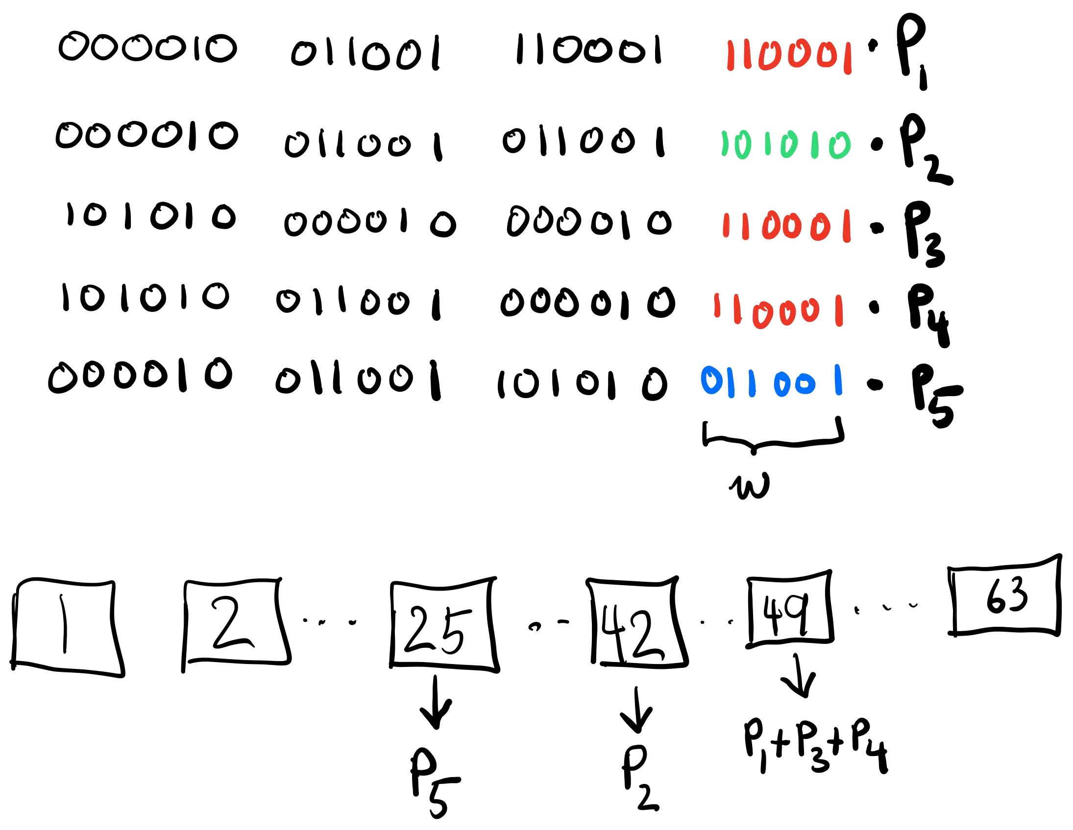
Then, for each window, we obtain a partial sum over the buckets

\[T_i = \sum_{k = 1}^{2^{w}-1} k B_k = B_1 + 2 B_2 + \dots + (2^w - 1)B_{2^w - 1}\]

In our example ($w = 6$) we have: $T_1 = 25P_5 + 42P_2 + 49(P_1 + P_3 + P_4)$.

The final value of the MSM is the radix-$2^w$ representation of the partial sums

\[T = \sum_{i = 1}^{\lambda/w} 2^{(i-1)w} T_i = T_1 + 2^w T_2 + 2^{2w} T_3 + \dots + 2^{(\frac{\lambda}{w}-1)w} T_{\lambda/w}\]

Where $\lambda$ is the bit length of our scalars ($24$ in this example). You’ll notice that both of these operations are themselves a multi-scalar multiplication. However, in practice we use an addition chain when iterating over the windows to avoid scalar multiplication all together.

Optimizations

1. Signed Scalar Representation

Point negation for short Weierstrass curves is cheap: $-(x, y) = (x, -y)$. We can cut our bucket list in half by normalizing our radix coefficients into the interval $[-2^{w-1}, 2^{w-1}]$. Then when we come across a negative coefficient we add $-P$ to $B_{|k|}$. This encoding can be precomputed at the beginning of the operation.

2. Parallelism

The partial sums $T_i$ are independent and can be computed concurrently. Enabling OpenMP support gives us an almost perfect linear speed up. The table below shows cycle counts for the same MSM computation with both implementations. Empirically, $4$ execution threads seem to give the best performance per point. This keeps all $4$ high performance cores busy.

$n$	blst	optimized	speedup
$2^{10}$	$29945$	$6415$	$4.7$x
$2^{11}$	$45161$	$8542$	$5.3$x
$2^{12}$	$73276$	$12670$	$5.8$x
$2^{13}$	$113445$	$21125$	$5.4$x